System Architecture

This chapter shows how the library, the simulation and the power stage model fit together, which data flows between them, and the development workflow that keeps them consistent. The individual modules are described in their own chapters.

The three repositories

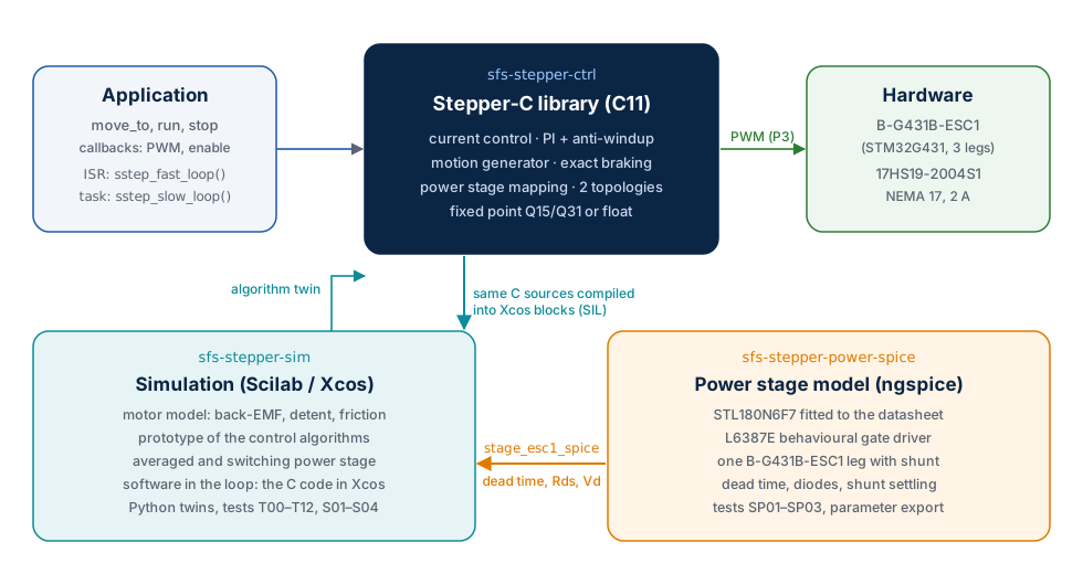
Part	Role in the system	Gives to the others	Takes from the others
Stepper-C (GitHub, folder sfs-stepper-ctrl)	The product: control loops for the MCU	C sources compiled into the Xcos blocks	Algorithms first proven in the prototype; dead time value for compensation
Simulation (sfs-stepper-sim)	Motor model, prototype of every algorithm, SIL test bench	Reference results, limits (speed, resonance, robustness)	The library sources (SIL); the switching stage parameters from ngspice
Power stage model (sfs-stepper-power-spice)	Transistor-level view of one ESC1 leg	params/stage_esc1_spice.sci / .json: effective dead time, leg resistance, diode drop	Board values (gate resistors, shunt, dead time)
Hardware (B-G431B-ESC1 + 17HS19-2004S1)	The target of the first port (P3)	Measured R, L, Kt, dead time, gate waveforms	The library and its configuration

The repositories are independent Git repositories that sit next to each other:

sfs-stepper/
├── sfs-stepper-ctrl/          Stepper-C library
├── sfs-stepper-sim/           Scilab/Xcos model, SIL, Python twins
├── sfs-stepper-power-spice/   ngspice model of the power stage
└── sfs-stepper-article/       this manual (website + PDF), repository Stepper-C-Motor-Control-Library

The simulation finds the library through the environment variable SSTEP_CTRL_DIR, a Git submodule ext/sfs-stepper-ctrl, or the sibling folder ../sfs-stepper-ctrl (in that order). The ngspice runner writes its export into ../sfs-stepper-sim/params/ when that folder exists.

Signal chain

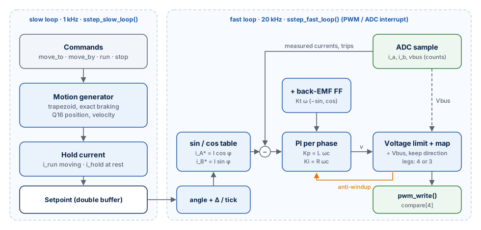
From a command to a turning shaft:

1. The application calls sstep_move_to() (or sstep_run(), sstep_stop()).
2. Every slow loop period (1 ms) the motion generator advances the position with the acceleration and velocity limits, chooses the current amplitude (run or hold) and publishes a setpoint: the electrical angle at the start of the period, its increment per fast period, the current amplitude and the back-EMF feed-forward.
3. Every fast loop period (50 µs at 20 kHz) sstep_fast_loop() converts the ADC counts to currents, checks the trip levels, computes the current references I cos φ, I sin φ, runs one PI controller per phase, adds the feed-forward, limits and maps the voltage vector to the legs of the topology and calls pwm_write().
4. The power stage applies the leg voltages; the motor turns the phase currents into torque; the ADC samples the currents at the centre of the next PWM period.

The same chain exists three times — in C (the library), in Scilab (the prototype) and in Python (the twin) — and the three are compared sample by sample.

How the parts are verified against each other

Comparison	Test	Agreement
Scilab motor model ↔ Python model (scipy, Radau)	X01	4·10⁻⁸ A
Scilab closed loop ↔ Python closed loop	X02, X03	5·10⁻¹³ A
Scilab motion generator ↔ C motion generator	tools/ref_motion.py against src/sstep_motion.c	bit-exact over 3 052 885 periods
C library in Xcos ↔ Scilab prototype	S01–S04	S02, S03: currents within 1.05 mA (ADC step 1.95 mA), commanded angle identical; S01, S04: re-run pending
Scilab switching stage ↔ Python switching stage ↔ C plant block	X04, host check	4·10⁻¹⁶ (C ↔ Python)
ngspice device model ↔ STL180N6F7 datasheet	SP01	Rds(on), Ciss, Coss, Crss, Qg within 10 %
C unit tests with a motor model ↔ Scilab prototype	gtest_sstep_loop.cpp	current step 1.11 % overshoot (prototype 1.12 %)

Development workflow

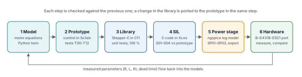
The work follows the order of the figure, and each step is checked against the previous one before the next starts:

1. Model. The motor equations are written once (stepper_motor_f) and checked against analytic results (T00–T02) and an independent Python solver (X01).
2. Prototype. Each control algorithm is first written in Scilab and tested on the model (T03–T12).
3. Library. The algorithm is implemented in C11 for both numeric backends, with unit tests and 100 % coverage.
4. Software in the loop. The C code runs in Xcos against the same model; S01–S04 must match the prototype.
5. Power stage. ngspice extracts the switching parameters of the real board; the simulation uses them.
6. Hardware. The library is ported to the B-G431B-ESC1; measured motor and board values flow back into the models.

Rule: the prototype follows the library

The Scilab prototype always implements the current algorithm of the library. A change in Stepper-C is ported to the prototype and to its Python twin in the same step, so that the SIL comparison compares identical algorithms.

Hardware reference

Item	Part	Key data
Motor	StepperOnline 17HS19-2004S1 (NEMA 17)	2 phases, 200 steps, 1.60 Ω, 3.0 mH, 2.0 A, 0.59 N·m, 82 g·cm²
Board	STMicroelectronics B-G431B-ESC1	STM32G431CB (Cortex-M4F, 170 MHz), 3 half-bridges, L6387E drivers, STL180N6F7 MOSFETs (60 V), three low-side shunts
Connection	Shared leg	phase A between U and W, phase B between V and W
Supply	Laboratory supply	24 V nominal (the board accepts 3S … 6S LiPo voltages)

With three legs the largest sinusoidal phase voltage is Vbus/√2 (17.0 V at 24 V) instead of Vbus with two H-bridges; the consequences are measured in Results.